『ゼロから作る Deep Learning』第4章 勉強メモ(最低限)

損失関数

ニューラルネットワークの性能の“悪さ”を示す指標で一般には、2 乗和誤差や交差エントロピー誤差などが用いられる

2 乗和誤差

E = ½ ∑ (y-t)²

def mean_squared_error(y, t):
  return 0.5 * np.sum((y-t)**2)
>>> # 「2」を正解とする
>>> t = [0, 0, 1, 0, 0, 0, 0, 0, 0, 0]
>>>
>>> # 例 1:「2」の確率が最も高い場合(0.6)
>>> y = [0.1, 0.05, 0.6, 0.0, 0.05, 0.1, 0.0, 0.1, 0.0, 0.0]
>>> mean_squared_error(np.array(y), np.array(t))0.097500000000000031

交差エントロピー誤差

E = -∑ t logy

def cross_entropy_error(y, t):
  delta = 1e-7
  return -np.sum(t * np.log(y + delta))

np.log(0) はマイナスの無限大を表す-inf となり、そ うなってしまうと、それ以上計算を進めることができなくなります。その防止策とし て、微小な値を追加して、マイナス無限大を発生させないようにしています。

>>> t = [0, 0, 1, 0, 0, 0, 0, 0, 0, 0]
>>> y = [0.1, 0.05, 0.6, 0.0, 0.05, 0.1, 0.0, 0.1, 0.0, 0.0]
>>> cross_entropy_error(np.array(y), np.array(t))
0.51082545709933802

訓練データすべての損失関数の平均

E = -1/N ∑ ∑ t logy (データが N 個)

[バッチ対応版]交差エントロピー誤差の実装

# データがひとつの場合と、データがバッチとしてまとめら れて入力される場合の両方のケースに対応
def cross_entropy_error(y, t):
  # yが普通の配列だったとき(データ一個の出力だったとき)行列にする
  if y.ndim == 1:
    t = t.reshape(1, t.size)
    y = y.reshape(1, y.size)
  # 出力した画像全てをまとめて損失関数の総和を出す
  # ちなみにy.shape[1]は出力層のニューロンの数
  batch_size = y.shape[0]
  return -np.sum(t * np.log(y)) / batch_size

ちなみにnp.sumや配列積は以下の例からわかるはず

>>> import numpy as np
>>> x = np.arange(10).reshape(2,5)
>>> y = np.arange(10).reshape(2,5)
>>> x
array([[0, 1, 2, 3, 4],
       [5, 6, 7, 8, 9]])
>>> x*y
array([[ 0,  1,  4,  9, 16],
       [25, 36, 49, 64, 81]])
>>> np.sum(x*y)
285

教師データがラベルとして与えられたとき(one-hot 表現ではなく、「2」や 「7」といったラベルとして与えられたとき)、交差エントロピー誤差は次のように実

装することができます

def cross_entropy_error(y, t):
  if y.ndim == 1:
    t = t.reshape(1, t.size)
    y = y.reshape(1, y.size)
  batch_size = y.shape[0]
  return -np.sum(np.log(y[np.arange(batch_size), t])) / batch_size

実装のポイントは、one-hot 表現で t が 0 の要素は、交差エントロピー誤差 も 0 であるから、その計算は無視してもよい。

y[np.arange(batch_size), t] は 各画像行 正解ラベル列として

array([ 画像1の正解ラベル出力値, 画像2の正解ラベル出力値, 画像3の正解ラベル出力値, ... , 画像Nの正解ラベル出力値 ])

になっている。

なぜ損失関数を設定するのか?

認識精度が高くなるようなパラメータ を獲得したいので、「認識精度」を指標にすべきではないか?

認識精度は離散値であり、微分がほとんどの場所で 0 になってし まい、パラメータの更新(学習)ができなくなってしまう。

例えば、訓練データが100枚の時、精度は1%毎にしか変化できない

微分

df(x)/dx = lim{(f(x + h) − f(x)) / h}

# 悪い実装例
def numerical_diff(f, x):
  h = 10e-50
  return (f(x+h) - f(x)) / h

h には 10e-50(「0.00...1」の 0 が 50 個続く数)という小さな値を用いてます。しかし、これでは逆に丸め誤差になる。

丸め誤差とは, 小数の小さな範囲において数値が省略され ることで(たとえば、小数点第 8 位以下が省略されるといったこと)、最終的な計算 結果に誤差が生じる

>>> import numpy as np
>>> np.float32(1e-50)
0.0

改善点1: 丸め誤差を避けるべく、微小な値 h として 10−4 を用いる。(10−4 程度 の値を用いれば、良い結果が得られることが分かってる。)

改善点2: (x, f(x)) (x+h, f(x+h)) の2点間の直線であり(前方差分)、接戦の傾きとは誤差があるので、誤差を減らす工夫とし て、(x + h) と (x − h) での関数 f の差分を計算する(中心差分)

def numerical_diff(f, x):
  h = 1e-4 # 0.0001
  return (f(x+h) - f(x-h)) / (2*h)

上記のように微小な差分によって微分を求めることを数値微分

一方、数式の展開によって微分を「解析的に解く」とか「解析的に微分を求める」などと言います

数値微分の例

(gradient_1d.py)
import numpy as np
import matplotlib.pylab as plt

def numerical_diff(f, x):
  h = 1e-4 # 0.0001
  return (f(x+h) - f(x-h)) / (2*h)

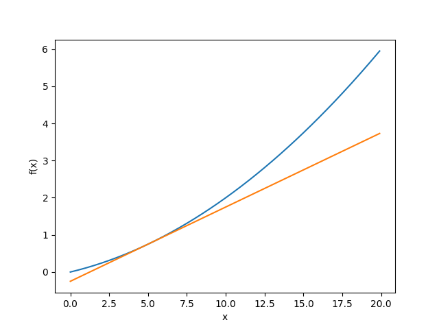
def function_1(x):
  return 0.01*x**2 + 0.1*x

def tangent_line(f, x):
  d = numerical_diff(f, x)
  print(d)
  # 接戦Y = dx + bより、以下はy切片bを表している
  b = f(x) - d*x
  # 傾きd y切片bの1次関数を返す関数を表している
  return lambda t: d*t + b

x = np.arange(0.0, 20.0, 0.1)
y = function_1(x) # 関数1
plt.xlabel("x")
plt.ylabel("f(x)")

tf = tangent_line(function_1, 5)
y2 = tf(x) # 接戦

plt.plot(x, y)
plt.plot(x, y2)
plt.show()

$ python gradient_1d.py
0.1999999999990898 # 真の微分は0.2なのでほとんど同じ値と見なすことができるぐらい小さな誤差

偏微分

f(x0,x1)=x0² +x1²

def function_2(x):
  return x[0]**2 + x[1]**2
  # または return np.sum(x**2)

x0 = 3、x1 = 4 のときの x0 に対する偏微分∂f / ∂x0

>>> def function_tmp1(x0):
... return x0*x0 + 4.0**2.0
...
>>> numerical_diff(function_tmp1, 3.0)6.00000000000378

x0 = 3、x1 = 4 のときの x1 に対する偏微分∂f / ∂x1

>>> def function_tmp2(x1):
... return 3.0**2.0 + x1*x1
...
>>> numerical_diff(function_tmp2, 4.0)7.999999999999119

(gradient_2d.py)
import numpy as np
import matplotlib.pylab as plt
from mpl_toolkits.mplot3d import Axes3D

# すべての変数の偏微分ベクトル(勾配)を求める
def _numerical_gradient_no_batch(f, x):
  h = 1e-4  # 0.0001
  grad = np.zeros_like(x) # xと形状が同じで値が全て0の配列

  for idx in range(x.size):
    tmp_val = x[idx]
    x[idx] = float(tmp_val) + h
    fxh1 = f(x)  # f(x+h)

    x[idx] = tmp_val - h
    fxh2 = f(x)  # f(x-h)
    grad[idx] = (fxh1 - fxh2) / (2*h)

    x[idx] = tmp_val  # 値を元に戻す
  return grad

# バッチ処理
def numerical_gradient(f, X):
  if X.ndim == 1:
    return _numerical_gradient_no_batch(f, X)
  else:
    grad = np.zeros_like(X)

  for idx, x in enumerate(X):
    grad[idx] = _numerical_gradient_no_batch(f, x)

  return grad


def function_2(x):
  if x.ndim == 1:
    return np.sum(x**2)
  else:
    return np.sum(x**2, axis=1)


def tangent_line(f, x):
  d = numerical_gradient(f, x)
  print(d) # 微分結果
  # 接戦のy切片d
  b = f(x) - d*x
  return lambda t: d*t + b


if __name__ == '__main__':
  x0 = np.arange(-2, 2.5, 0.25)
  x1 = np.arange(-2, 2.5, 0.25)
  X, Y = np.meshgrid(x0, x1)

  X = X.flatten()
  Y = Y.flatten()

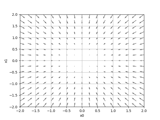
  grad = numerical_gradient(function_2, np.array([X, Y]).T).T

  plt.figure() # Figureインスタンスを作成
  plt.quiver(X, Y, -grad[0], -grad[1],  angles="xy",color="#666666") # 矢印（ベクトル）
  plt.xlim([-2, 2])
  plt.ylim([-2, 2])
  plt.xlabel('x0')
  plt.ylabel('x1')
  plt.grid()
  plt.draw()
  plt.show()

補足: enumerate 

Pythonのenumerate()関数を使うと、forループの中でリスト（配列）などのイテラブルオブジェクトの要素と同時にインデックス番号（カウント、順番）を取得できる。

l = ['Alice', 'Bob', 'Charlie']
for i, name in enumerate(l):
    print(i, name)
# 0 Alice
# 1 Bob
# 2 Charlie

補足: np.ndarray.flatten 多次元配列を一次元配列

>>> x=np.arange(12).reshape(2,3,2)
>>> x.flatten()
array([ 0,  1,  2,  3,  4,  5,  6,  7,  8,  9, 10, 11])

補足: meshgridについて

例えばx = [1,2,3,4,5,6,7,8,9]の配列をX軸y = [10,20,30,40,50]の配列をY軸として表を作る場合

上のような表の各要素のx値とy値から各要素に入る値を求めることになる。

meshgrid() を使うと、予め上のような表（実際は行列）に各要素毎のx値とy値を埋めたものを生成してくれる。

import numpy as npx = [1,2,3,4,5,6,7,8,9]

y = [10,20,30,40,50]

X,Y = np.meshgrid(x,y)

print(X)

# => [[1 2 3 4 5 6 7 8 9]

#    [1 2 3 4 5 6 7 8 9]

#    [1 2 3 4 5 6 7 8 9]

#    [1 2 3 4 5 6 7 8 9]

#    [1 2 3 4 5 6 7 8 9]]

print(Y)

# => [[10 10 10 10 10 10 10 10 10]

#     [20 20 20 20 20 20 20 20 20]

#     [30 30 30 30 30 30 30 30 30]

#     [40 40 40 40 40 40 40 40 40]

#     [50 50 50 50 50 50 50 50 50]]

このような座標行列を予め作成しておくことより、
例えば
f(x,y) = x+yの値を求める場合

print(X+Y)

# => [[11 12 13 14 15 16 17 18 19]

#     [21 22 23 24 25 26 27 28 29]

#     [31 32 33 34 35 36 37 38 39]

#     [41 42 43 44 45 46 47 48 49]

#     [51 52 53 54 55 56 57 58 59]]

f(x,y) = x+2yの場合は

print(X+2*Y) 

# => [[ 21 22 23 24 25 26 27 28 29] 

#     [ 41 42 43 44 45 46 47 48 49] 

#     [ 61 62 63 64 65 66 67 68 69] 

#     [ 81 82 83 84 85 86 87 88 89] 

#     [101 102 103 104 105 106 107 108 109]]

のようにシンプルに各座標値を求めることができます。

補足: plt.quiver ベクトル(矢印)について

plt.quiver(0.5,0.5,0.5,0.5) #(x,y,u,v) x,y-始点座標、u,v-ベクトルの向き

わかりやすかった参考文献 https://algorithm.joho.info/programming/python/matplotlib-quiver/

$ python gradient_2d.py

勾配法

最小値を探す場合を勾配降下法(gradient descent method)、最大値を探す場合を勾配上昇法(gradient ascent method)と言います。

一般的に、ニューラルネットワーク(ディー プラーニング)の分野では、勾配法は「勾配降下法」として登場

x0 = x0 - η (∂f / ∂x0)

η は学習率と呼ばれ、

学習率の値は、0.01 や 0.001 など、前もって何らかの値に決める必要がある。一般的に、大きすぎても小さすぎても、「良い場所」にたどり着くことができない。

# lr(learningrate)学習率, step_num 学習回数
def gradient_descent(f, init_x, lr=0.01, step_num=100):
  x  = init_x
  for i in range(step_num):
    grad = numerical_gradient(f, x)
    x -= lr * grad
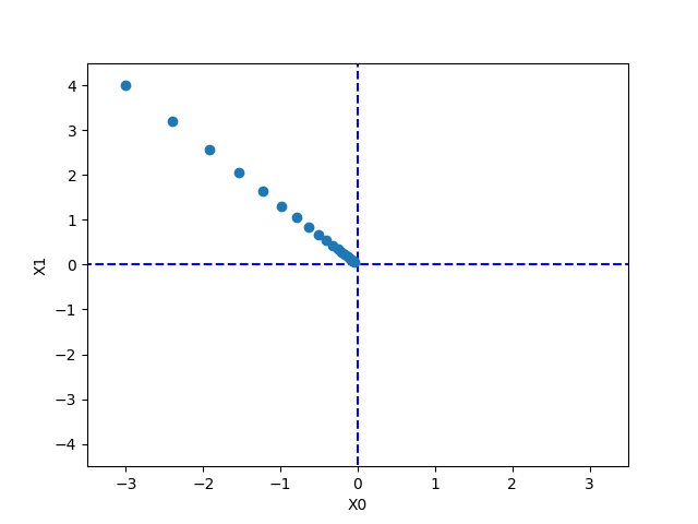
  return x

問: f(x0 , x1 ) = x0² + x1² の最小値を勾配法で求めよ

>>> def function_2(x):
...   return x[0]**2 + x[1]**2...

>>>  init_x = np.array([-3.0, 4.0])
>>>  gradient_descent(function_2, init_x=init_x, lr=0.1, step_num=100)
array([ -6.11110793e-10, 8.14814391e-10])

最終的な結果は (-6.1e-10, 8.1e-10) となり、これはほとんど (0, 0)に近い。

真の最小値は (0, 0) なので、勾配法によって、ほぼ正 しい結果を得ることができた

(gradient_method.py)
import numpy as np
import matplotlib.pylab as plt
from gradient_2d import numerical_gradient


def gradient_descent(f, init_x, lr=0.01, step_num=100):
  x = init_x
  x_history = []

  for i in range(step_num):
    x_history.append( x.copy() ) # 配列に要素を追加
    grad = numerical_gradient(f, x)
    x -= lr * grad
  return x, np.array(x_history)


def function_2(x):
  return x[0]**2 + x[1]**2

init_x = np.array([-3.0, 4.0])    
lr = 0.1
step_num = 20
x, x_history = gradient_descent(function_2, init_x, lr=lr, step_num=step_num)
#print("学習結果x")
#print(x)
#print("学習過程")
#print(x_history)

plt.plot( [-5, 5], [0,0], '--b') # blue markers with default shape
plt.plot( [0,0], [-5, 5], '--b')
plt.plot(x_history[:,0], x_history[:,1], 'o') # 'o' サークルマーカー

plt.xlim(-3.5, 3.5)
plt.ylim(-4.5, 4.5)
plt.xlabel("X0")
plt.ylabel("X1")
plt.show()

補足: array.copy() オブジェクトをコピーする(値を参照ではなく全く別のものを複製)

・値渡しと参照渡し

参照渡し
>>> x=[1,2,3]
>>> y=x
>>> y.apend(4)
>>> y,x
[1, 2, 3, 4], [1, 2, 3, 4]

上記は参照元と参照先がメモリを共有した状態であり、一方を変更したら両方変更が適用される

値渡し
>>> x=[1,2,3]
>>> y=x.copy()
>>> y.append(4)
>>> x,y
([1, 2, 3], [1, 2, 3, 4])

補足: matplotlib.pyplot.plotのオプションいついてはドキュメント参照

https://translate.google.com/translate?hl=ja&sl=en&u=https://matplotlib.org/3.1.0/api/_as_gen/matplotlib.pyplot.plot.html&prev=search

補足: array[:,0]やarray[:,1]について

[行:列]でスライスでき、省略した場合はすべてを指定したことになるので、[:, 0]は全ての行の0列目を取得することになります。省略せずに書くと2x2の配列の場合ならa[0:2, 0]となります。

>>> a = numpy.array([[0,1], [2, 3]])
>>> aarray([[0, 1],       [2, 3]])
>>> a[:,0]array([0, 2])
>>>

$ python gradient_method.py

簡単なニューラルネットワークを例にして、実際に勾配を求める実装

(gradient_simplenet.py)
import sys, os 
sys.path.append(os.pardir)
import numpy as np from common.functions 
from common.functions import softmax, cross_entropy_error 
from common.gradient import numerical_gradient
class simpleNet:    
  def __init__(self):
    self.W = np.random.randn(2,3) # ガウス分布で重み初期化

  def predict(self, x):
      return np.dot(x, self.W)

  def loss(self, x, t):
    z = self.predict(x)
    y = softmax(z)
    loss = cross_entropy_error(y, t)
    return loss

x = np.array([0.6, 0.9])
t = np.array([0, 0, 1])

net = simpleNet()

f = lambda w: net.loss(x, t)
dW = numerical_gradient(f, net.W)

print(dW) # 重みの微分結果

学習アルゴリズムの実装

2 層ニューラルネットワークを、ひとつのクラスとして実装する

(two_layer_net.py)
import sys, os
sys.path.append(os.pardir)  # 親ディレクトリのファイルをインポートするための設定
from common.functions import *
from common.gradient import numerical_gradient

class TwoLayerNet:
  # 引数は、入力層のニューロンの数、隠れ層のニューロンの数、出力層のニューロンの数
  def __init__(self, input_size, hidden_size, output_size, weight_init_std=0.01):
  # 重みの初期化
    self.params = {}
    self.params['W1'] = weight_init_std * np.random.randn(input_size, hidden_size)
    self.params['b1'] = np.zeros(hidden_size)
    self.params['W2'] = weight_init_std * np.random.randn(hidden_size, output_size)
    self.params['b2'] = np.zeros(output_size)

  # 入力層のニューロンからニューラルネットワークの計算値を出力
  def predict(self, x):
    W1, W2 = self.params['W1'], self.params['W2']
    b1, b2 = self.params['b1'], self.params['b2']

    a1 = np.dot(x, W1) + b1
    z1 = sigmoid(a1)
    a2 = np.dot(z1, W2) + b2
    y = softmax(a2)
    return y

  # 損失関数を求める x:入力データ, t:教師データ
  def loss(self, x, t):
    y = self.predict(x)
    return cross_entropy_error(y, t)

  # 認識精度(0~1)
  def accuracy(self, x, t):
    y = self.predict(x)
    y = np.argmax(y, axis=1)
    t = np.argmax(t, axis=1)
    accuracy = np.sum(y == t) / float(x.shape[0])
    return accuracy

  # 重みパラメータに対する勾配を求める x:入力データ, t:教師データ
  def numerical_gradient(self, x, t):
    loss_W = lambda W: self.loss(x, t)
    # 勾配を保持するディクショナリ変数
    grads = {}
    grads['W1'] = numerical_gradient(loss_W, self.params['W1'])
    grads['b1'] = numerical_gradient(loss_W, self.params['b1'])
    grads['W2'] = numerical_gradient(loss_W, self.params['W2'])
    grads['b2'] = numerical_gradient(loss_W, self.params['b2'])
    return grads

  # 重みパラメータに対する勾配を求める numerical_gradient() の高速版!
  def gradient(self, x, t):
    W1, W2 = self.params['W1'], self.params['W2']
    b1, b2 = self.params['b1'], self.params['b2']
    grads = {}

    batch_num = x.shape[0]

    # forward
    a1 = np.dot(x, W1) + b1
    z1 = sigmoid(a1)
    a2 = np.dot(z1, W2) + b2
    y = softmax(a2)

    # backward
    dy = (y - t) / batch_num
    grads['W2'] = np.dot(z1.T, dy) # 2層目の重みの勾配
    grads['b2'] = np.sum(dy, axis=0) # 二層目のバイアスの勾配

    dz1 = np.dot(dy, W2.T)
    da1 = sigmoid_grad(a1) * dz1
    grads['W1'] = np.dot(x.T, da1) # 1層目の重みの勾配
    grads['b1'] = np.sum(da1, axis=0) # 一層目のバイアスの勾配

    return grads

TwoLayerNet クラスを対象に、MNIST データセッ トを使って学習

(train_nueralnet.py)
# coding: utf-8
import sys, os
sys.path.append(os.pardir)  # 親ディレクトリのファイルをインポートするための設定
import numpy as np
import matplotlib.pyplot as plt
from dataset.mnist import load_mnist
from two_layer_net import TwoLayerNet

# データの読み込み
(x_train, t_train), (x_test, t_test) = load_mnist(normalize=True, one_hot_label=True)

network = TwoLayerNet(input_size=784, hidden_size=50, output_size=10)

iters_num = 10000  # 勾配法による更新の回数(繰り返し回数)を適宜設定する
train_size = x_train.shape[0]
batch_size = 100
learning_rate = 0.1

train_loss_list = []
train_acc_list = []
test_acc_list = []

# 1エポックあたりの繰り返し数(訓練データの総数6万枚に相当する量を読み込んだ時全ての画像を見たと定め1エポック)
iter_per_epoch = max(train_size / batch_size, 1)
count=0
for i in range(iters_num):
  # ミニバッチの取得
  batch_mask = np.random.choice(train_size, batch_size) # train_size未満の自然数をbatch_size個セレクト
  x_batch = x_train[batch_mask] # 例えば, x_train[[0,3]] だったら[x_train[0],x_train[3]] になる
  t_batch = t_train[batch_mask]

  # 勾配の計算
  #grad = network.numerical_gradient(x_batch, t_batch)
  grad = network.gradient(x_batch, t_batch)

  # パラメータの更新(学習)
  for key in ('W1', 'b1', 'W2', 'b2'):
    network.params[key] -= learning_rate * grad[key]

  # 損失関数を計算して配列にメモ
  loss = network.loss(x_batch, t_batch)
  train_loss_list.append(loss)

  # 1エポック(バッチ)ごとに認識精度を計算 今回はiter_per_epochが600.0なので600回ごとに実行される
  if i % iter_per_epoch == 0:
    # print(i) => 0,600,1200, ... ,9600
    train_acc = network.accuracy(x_train, t_train)
    test_acc = network.accuracy(x_test, t_test)
    train_acc_list.append(train_acc) # 精度をメモ
    test_acc_list.append(test_acc) # 精度をメモ
    print("train acc, test acc | " + str(train_acc) + ", " + str(test_acc))

  # グラフの描画
markers = {'train': 'o', 'test': 's'}
x = np.arange(len(train_acc_list))
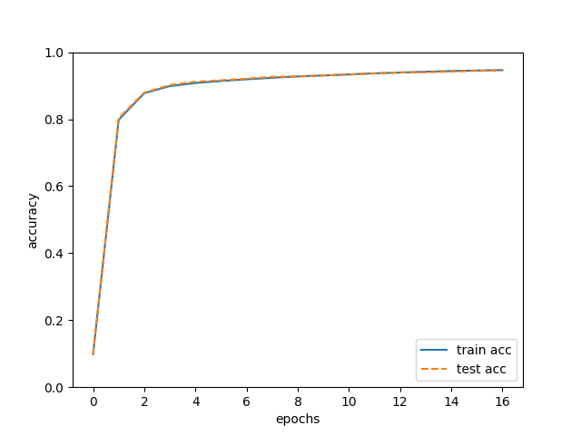
plt.plot(x, train_acc_list, label='train acc')
plt.plot(x, test_acc_list, label='test acc', linestyle='--')
plt.xlabel("epochs")
plt.ylabel("accuracy")
plt.ylim(0, 1.0)
plt.legend(loc='lower right')
plt.show()

$ python train_neuralnet.py
train acc, test acc | 0.09871666666666666, 0.098
train acc, test acc | 0.7983166666666667, 0.8035
train acc, test acc | 0.8775833333333334, 0.8794
train acc, test acc | 0.8989, 0.902
train acc, test acc | 0.9080333333333334, 0.9117
train acc, test acc | 0.9140666666666667, 0.9162
train acc, test acc | 0.91905, 0.9208
train acc, test acc | 0.92365, 0.9265
train acc, test acc | 0.9277333333333333, 0.9272
train acc, test acc | 0.9306166666666666, 0.9305
train acc, test acc | 0.9336333333333333, 0.9334
train acc, test acc | 0.9368166666666666, 0.9366
train acc, test acc | 0.93925, 0.9399
train acc, test acc | 0.9417333333333333, 0.9401
train acc, test acc | 0.9438833333333333, 0.942
train acc, test acc | 0.9452666666666667, 0.9444
train acc, test acc | 0.9467, 0.9455

学習をしていない初めは確率通りでほぼ10%であり、6万枚を16エポック96万枚学習した性能は94%である

訓練データとテストデータを使って評価した認識精度は両方とも向上している。

また、その 2 つの認識精度には差がないことが分かる(その 2 つの線はほぼ重なっている)。

そのため、今回の学習では過学習が起きていないことが 分かる。